User Manual¶

Welcome to the user manual for SETLyze. This manual explains the usage of SETLyze.

Introduction¶

SETLyze is a part of the SETL project, a fouling community study focussing on marine invasive species. The website describes the SETL project as follows:

“Over the last ten years, marine invaders have had a dramatically increasing impact on temperate water ecosystems around the world. Substantial ecological and economical damage has been caused by the introduction of diseases, parasites, predators, invaders outcompeting native species, and species that are a nuisance for public health, tourism, aquaculture or in any other way. In the SETL-project standardized PVC-plates are used to detect these invasive species and other fouling community organisms. The material and methods of the SETL-project were developed by the ANEMOON foundation in cooperation with the Smithsonian Marine Invasions Laboratory of Smithsonian Environmental Research Centre. In this project 14x14 cm PVC-plates are hung 1 meter below the water surface, and refreshed and checked for species at least every three months.” — ANEMOON foundation

Data collected from these SETL plates are stored in the SETL database. This database currently contains over 25000 records containing information of over 200 species in different locations throughout the Netherlands. SETLyze is an application capable of performing a set of analyses on this SETL data. SETLyze can perform the following analyses:

Spot Preference: Determine a species’ preference for a specific location on a SETL plate. Species can be combined so that they are treated as a single species.
Attraction within Species: Determine if a species attracts or repels individuals of its own kind. Species can be combined so that they are treated as a single species.
Attraction between Species: Determine if two different species attract or repel each other. Species can be combined so that they are treated as a single species.

Additionally, any of the above analyses can be performed in batch mode, meaning that the analysis is repeated for each species of a species selection. Thus an analysis can be easily performed on an entire data set without intervention. Batch mode for analyses are parallelized such that the computing power of a computer is optimally used.

Data Collection¶

First let’s have a look at how the data for the SETL project is being collected. When the SETL plates are checked, each plate is first carefully pulled out of the water and then photographed. This is done by a standard procedure described on the ANEMOON foundation’s website. First an overview photograph is taken of each plate. Then some more detailed photographs are taken of the species that grow on each plate. Indivdual plates are recognized by their tags. The pictures are then carefully analyzed. For each plate the SETL-monitoring form is filled in. For each species the absence or presence, abundance and area cover are filled in. For this, a 5x5 grid is digitally applied over the photograph (SETL plate with digitally applied grid). For each species the presence or absence on each of the 25 plate surfaces are filled in and saved to the database.

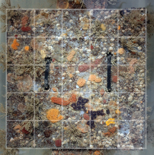
SETL plate with digitally applied grid

Each record in the database contains a species ID, a plate ID, and the 25 plate surfaces. The species ID links to the species that was found on the plate. The plate ID links to the plate on which that species was found. The plate ID is also linked to the location where this plate was deployed. The 25 plate surfaces (“spots”) are stored in each record as booleans (meaning they can have a value of True or False). The value 1 (True) for a spot means that the species in question was present on that spot of the plate. The value 0 (False) means that the species was absent from that spot.

With 25 spots x 2500 records = 625000+ booleans for the presence/absence of species, automatic methods of analyzing this data are required. Hence SETLyze was developed, a tool for analyzing the settlement of species on SETL plates.

Using SETLyze¶

SETLyze comes with a graphical user interface (GUI). The GUI consists of dialogs which all have a specific task. These dialogs will guide you in performing the set of analyses it provides. Most of SETLyze’s dialogs have a Help button which when clicked should point you to the corresponding dialog description on this page. All dialog descriptions can be found in the SETLyze dialogs section of this manual.

Before SETLyze can perform an analysis it needs access to a data source containing SETL data. Currently two data sources are supported: Text (.csv) or Excel (.xls) files exported from the Microsoft Access SETL database. This means that the user must first export the tables of the SETL database from Microsoft Access to these files. This would result in four files, one for each table. The user is then required to load these files into SETLyze. First follow the steps to export the SETL data.

You can perform an analysis once you have loaded the four data files containing the SETL data. Start SETLyze and you should be presented with the Analysis Selection dialog. Select an analysis and press OK to begin. A new dialog will be displayed, most likely the Locations Selection dialog.

If this is your first time running SETLyze, the locations selection dialog will show an empty locations list because no data has been loaded yet. To load SETL data, click on the Change Data Source button to open the change data source dialog. This dialog allows you to load data from CSV or XLS files exported from the Microsoft Access SETL database.

Once the data has been loaded, the locations selection dialog will automatically update the list of locations. From here on it’s just a matter of following the instruction one the screen. Should you need more help, scroll down to the SETLyze dialogs section for a more extensive description of each dialog. The dialog descriptions are also accessible from SETLyze’s dialogs itself by clicking the Help button on a dialog.

Definition List¶

This part of the user manual describes some terminology often used throughout the application and this manual.

Intra specific: Within a single species.
Inter specific: Between two different species.

Plate area

The defined area on a SETL plate. By default the SETL plate is divided in four plate areas (A, B, C and D):

Default plate areas

Plate areas can be customized during an analysis, see Define Plate Areas dialog.

Positive spot: Each record in the SETL database contains data for each of the 25 spots on a SETL plate. The spots are stored as booleans, meaning they can have two values; 1 (True) means that the species was present on that spot, 0 (False) means that the species was absent on that spot. A spot is “positive” if the spot value is 1 or True. Each record can thus have up to 25 positive spots.
SETL plate: In the SETL project standardized PVC-plates are used to detect invasive species and other fouling community organisms. In this project 14x14 cm PVC-plates are hung 1 meter below the water surface, and refreshed and checked for species at least every three months.
Spot: To analyze SETL plates, photographs of the plates are taken. The photographs are then analyzed on the computer by applying a 5x5 grid to the photographs. This divides the SETL plate into 25 equal surface areas (see SETL plate with digitally applied grid). Each of the 25 surface areas are called “spots”. Species are scored for presence/absence for each of the 25 spots on each SETL plate, and the data is stored in the SETL database in the form of records. So each SETL record in the database contains presence/absence data of one species for all 25 spots on a SETL plate.

Spot distance

Spot distances are the distances between positive spots on a SETL plate. The spot distances are calculated from observed and expected positive spots data and are used to define whether species attract or repel.

Observed spot distances (intra specific)

All possible distances between the spots on each plate are calculated using the Pythagorean theorem. Consider the case of species A and the following plate:

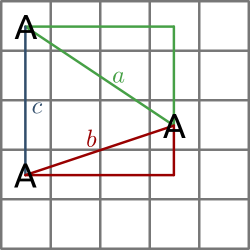
Spot distances on SETL plate (intra specific)

As you can see from the figure, three positive spots results in three spot distances (a, b and c). The distance from one spot to the next by moving horizontally or vertically is defined as 1. The distances from the figure are calculated as follows:

$spot\_distance(a) = \sqrt{3^2 + 2^2} = 3.61$

$spot\_distance(b) = \sqrt{3^2 + 1^2} = 3.16$

$spot\_distance(c) = \sqrt{0^2 + 3^2} = 3$

This is done for all plates of an analysis. Note that there can be no distance 0, in contrast to inter specific spot distances (see below).

Observed spot distances (inter specific)

To obtain spot distances for analyses where two species are involved, first the plate records are collected that contain both of the selected species. Then all possible spot distances are calculated between the two species. The following figure shows an example with positive spots for two species (A and B) and all possible spot distnaces.

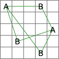
Spot distances on SETL plate (inter specific)

In the above figure, the distances are calculated the same way as for intra specific spot distances. Note however that only inter specific distances are calculated (distances between two different species). This also makes it possible to have a distance of 0 as visualized in the next figure.

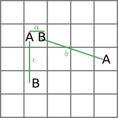
Spot distances on SETL plate (inter specific)

The distances for this figure are calculated as follows:

$spot\_distance(a) = \sqrt{0^2 + 0^2} = 0$

$spot\_distance(b) = \sqrt{3^2 + 1^2} = 3.16$

$spot\_distance(c) = \sqrt{0^2 + 2^2} = 2$

Expected spot distances

The expected spot distances are calculated by generating a copy of each plate record matching the species selection. Each copy has the same number of positive spots as its original, except the positive spots are placed randomly at the plates. Then the spot distances are calculated the same way as for the observed spot distances. This means that the resulting list of expected spot distances has the same length as the observed spot distances.

SETLyze dialogs¶

SETLyze comes with a graphical user interface consisting of separate dialogs. The dialogs are described in this section.

Analysis Selection dialog¶

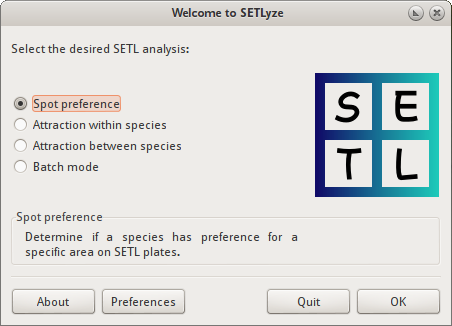
Analysis Selection dialog

The analysis selection dialog is the first dialog you see when SETLyze is started. It allows the user to select an analysis to perform on SETL data. The user can select one of the analyses in the list and click on the OK button to start the analysis. Clicking the Quit button closes the application.

After pressing the OK button, two things can happen. If no SETL data was found on the user’s computer, SETLyze automatically tries to load SETL locations and species data from the SETL database server. This requires a direct connection with the SETL database server. A progress dialog is shown while the data is being loaded. If connecting to the database server fails, SETLyze continues without data. Since the database server has not been implemented yet, no data will be loaded.

If SETL data is found on the user’s computer, an information dialog is displayed telling the user that existing data is being loaded.

Clicking the About button shows SETLyze’s About dialog. The About dialog shows general information about SETLyze; its version number, license information, a link to the GiMaRIS website, the application developers, and contact information.

Clicking the Preferences button loads the Preferences dialog.

Batch Mode dialog¶

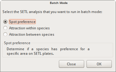
Batch Mode dialog

Selecting “Batch mode” in the Analysis Selection dialog brings up the Batch Mode dialog. This dialog allows you to start an analysis in batch mode. In batch mode, the selected analysis is repeated for each species in a species selection (or each inter species combination for analysis “Attraction between Species”). When multiple species are selected the analysis is repeated for each species separately and the results are displayed in a Summary Report. The summary report only displays the species that had significant results.

Preferences dialog¶

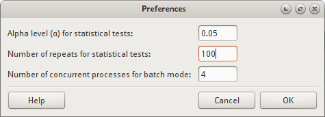
Preferences dialog

The preferences dialog allows you to change SETLyze’s settings. Settings set here are saved to a configuration file in the user’s home directory (~/.setlyze/setlyze.cfg). The following settings can be changed:

Alpha level (α) for statistical tests

Sets the alpha level. The alpha level must be a number between 0 and 1. The default value 0.05 means an alpha level of 5%.

This alpha level is translated to a confidence level with the formula $conf. level = 1 - \alpha$ . This confidence level is used for some statistical tests to calculate the confidence interval. At this moment this is just the t-test (not used in any analysis at this point).

The alpha level is also used to determine if a P-value returned by statistical tests is considered significant. The P-value is considered significant if the P-value is equal or less than the alpha level.

Number of repeats for statistical tests

Sets the number of repeats to perform on some statistical tests. Some statistical tests used in SETLyze use expected values that are randomly generated. This means you can’t draw a solid conclusion from the result of just one test. There is a change that the found result was a coincidence. To account for this, these test are repeated a number of times. The default value is 20 repeats. This value is very low, but good enough for testing purposes. When you need to draw solid conclusions, this value needs to be set to a higher number.

Number of concurrent processes for batch mode

Batch mode for analyses are parallelized which means that multiple analyzes can be executed in parallel. The value set here corresponds to the number of concurrent processes that will execute analyses. The higher the number, the faster a batch analysis will complete. The number of processes must be at least 1 and no more than the number of CPUs. The default value of this option equals to 90% of the available CPUs.

Locations Selection dialog¶

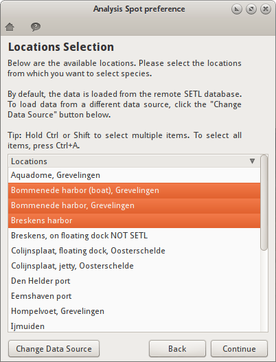
Locations Selection dialog

The locations selection dialog shows a list of all SETL locations. This dialog allows you to select locations from which you want to select species. The Species Selection dialog (displayed after clicking the Continue button) will only display the species that were recorded in the selected locations. Subsequently this means that only the SETL records that match both the locations and species selection will be used for the analysis, as each SETL record is bound to a species and a SETL plate from a specific location.

The Change Data Source button opens the Load Data dialog. This dialog allows you to load new SETL data. After doing so, the locations selection dialog is automatically updated with the new data.

The Back button allows you to go back to the previous dialog. This can be useful when you want to correct a choice you made in a previous dialog.

The Continue button saves the selection, closes the dialog, and shows the next dialog.

Making a selection¶

Just click on one of the locations to select it. To select multiple locations, hold Ctrl or Shift while selecting. To select all locations at once, click on a location and press Ctrl+A.

Species Selection dialog¶

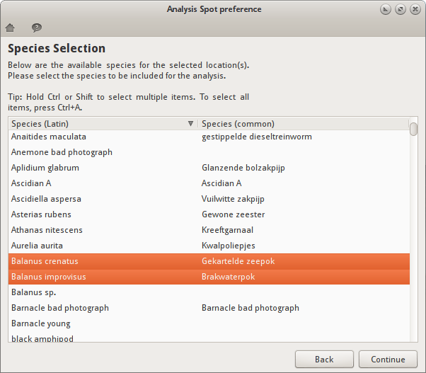
Species Selection dialog

The species selection dialog shows a list of all SETL species that were found in the selected SETL locations. This dialog allows you to select the species to be included in the analysis. Only the SETL records that match both the locations and species selection will be used for the analysis.

It is possible to select more than one species (see Making a selection). Selecting more than one species in a single species selection dialog means that the selected species are threated as one species for the analysis. In batch mode however, the analysis is repeated for each of the selected species.

If the selected analysis requires two or more separate species selections (e.g. two species are compared), it will display the selection dialog multiple times. In this case, the header of the selection dialog will say “First Species Selection”, “Second Species Selection”, etc.

The Back button allows you to go back to the previous dialog. This can be useful when you want to correct a choice you made in a previous dialog.

The Continue button saves the selection, closes the dialog, and shows the next dialog.

Making a selection¶

Just click on one of the species to select it. To select multiple species, hold Ctrl or Shift while selecting. To select all species at once, click on a species and press Ctrl+A.

Load Data dialog¶

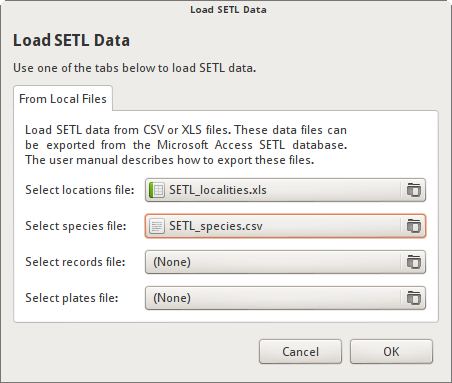
Load Data dialog

The Load Data dialog allows you to load SETL data into SETLyze. Two data sources are supported:

Text CSV (*.csv, *.txt) files exported from the Microsoft Access SETL database. The CSV files need to be exported by Microsoft Access, one file for each of the four tables: SETL_localities, SETL_plates, SETL_records, and SETL_species. The section Exporting SETL data from the Access database describes how to export these files.
Excel 97/2000/XP/2003 (*.xls) files exported from the Microsoft Access SETL database. One file for each of the four tables: SETL_localities, SETL_plates, SETL_records, and SETL_species. Microsoft Access by default includes a header row in the exported XLS files. The header row must be removed before importing into SETLyze.

After selecting all four data files files, press the OK button to load the SETL data from these files. A progress dialog is shown while the data is being loaded. Once the data has been loaded, the Locations Selection dialog will be updated with the new data.

Define Plate Areas dialog¶

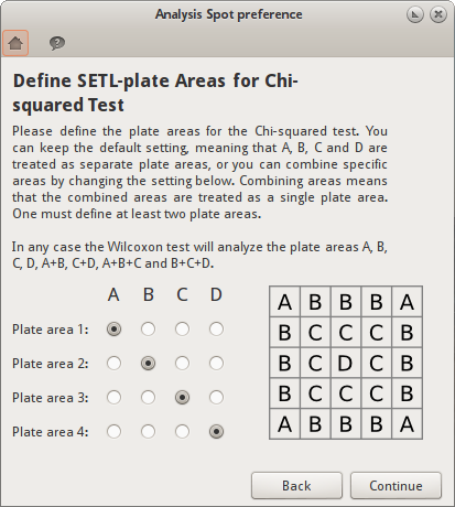
Define Plate Areas dialog

This dialog allows you to define the plate areas for analysis “Spot Preference”. By default, the SETL plate is divided in four plate areas: A, B, C and D. This dialog allows you to combine these areas by changing the area definitions. Combining areas means that the combined areas are treated as a single plate area. One must define at least two plate areas.

The user defined plate areas are only used for the Chi-squared test. In any case the Wilcoxon test will analyze the plate areas A, B, C, D, A+B, C+D, A+B+C and B+C+D.

Below is a schematic SETL plate with a grid. By default the plate is divided in four plate areas (A, B, C and D),

Default plate areas

But sometimes it’s useful to combine plate areas. So if one decides to combine areas A and B, the selection could be changed as follows,

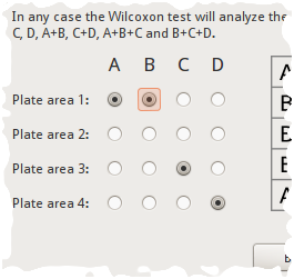
Combined plate areas selection

And the resulting plate areas definition would look something like this,

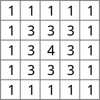
Plate areas A and B combined.

This would result in three plate areas. Analysis “Spot Preference” would then determine if the selected species has a preference for either of the three plate areas.

The names of the plate areas (area 1, area 2, ...) do not have a special meaning. It is simply used internally by the application to distinguish between plate areas. These area names are also used in the analysis report to distinguish between the plate areas.

The Back button allows you to go back to the previous dialog. This can be useful when you want to correct a choice you made in a previous dialog.

The Continue button saves the selection, closes the dialog, and shows the next dialog.

Analysis Report dialog¶

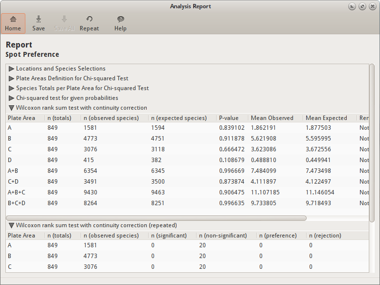
Analysis Report dialog

The analysis report dialog shows the results for an analysis. The dialog consists of the results frame and a toolbar on top. The toolbar holds a number of buttons. Hover your mouse pointer over the buttons to reveal a tooltip which explains the button’s action. Some buttons are explained below:

Save

The “Save” button allows you to save the report to a file. Clicking this button first shows a File Save dialog which allows you to select a target directory and filename. One file type is supported:

reStructuredText (*.rst) - Plain text files in an easy-to-read markup syntax. One can use Docutils to convert reStructuredText files into useful formats, such as HTML, LaTeX, man-pages, open-document or XML.

Save All

The “Save All” button is only enabled in batch mode and allows you to export the reports of the individual analyses. Clicking the “Save” button in batch mode only saves the Summary Report which is based on the individual reports.

Repeat

The “Repeat” button can be used to repeat an analysis with different parameters. Clicking this button will open a dialog which shows the same parameters available in the Preferences dialog. So one can, for example, quickly repeat the analysis with a different number of repeats.

The report dialog can display two types of reports:

Standard Report: When running an analysis in standard mode (not in batch mode) the report is divided into sections. There is a section for each statistical test that was performed.
Summary Report: When running an analysis in batch mode the report will be a summary of all standard reports that were generated. This report will show less details than a standard report.

Both types of reports will be explained below.

Standard Report¶

A standard report is divided into subsections. You have to click on a subsection to reveal its contents. Find the explanation for each subsection below.

Locations and Species Selections¶

Displays the locations and species selections. If multiple selections were made, each element is suffixed by a number. For example “Species selection (2)” stands for the second species selection.

Wilcoxon rank sum test with continuity correction¶

Shows the results for the non-repeated Wilcoxon rank-sum tests.

“In statistics, the Mann–Whitney U test (also called the Mann–Whitney–Wilcoxon (MWW) or Wilcoxon rank-sum test) is a non-parametric statistical hypothesis test for assessing whether two independent samples of observations have equally large values.” — Mann–Whitney U (Wikipedia. 6 December 2010)

Tests showed that spot distances on a SETL plate are not normally distributed (see Testing spot distances for normal distribution), hence the Wilcoxon rank-sum test for unpaired data was chosen to test if observed and expected spot distances differ significantly. The observed and expected spot distances

Depending on the analysis, the test is performed on different groups of data. The data can be grouped by plate area (analysis “Spot Preference”), the number of positive spots (analysis “Attraction within Species”) or by positive spot ratios groups (analysis “Attraction between Species”). See section record grouping for more information on data grouping.

Each row for the results of the Wicoxon test contains the results of a single test on a data group. Each row can have the following elements:

Plate Area: The plate area of a SETL plate. A SETL plate is divided into four plate areas: A, B, C, and D (see Default plate areas). The test is performed on each of the four plate areas, plus the combinations “A+B”, “C+D”, “A+B+C”, and “B+C+D”. Combining the results of the test for all plate areas (and combinations) allows you to make conclusions about the species’ preference for areas on SETL plates. See also Grouping by Plate Area.
Positive Spots: A number representing the number of positive spots. For this test only records matching that number of positive spots were used. See also Record grouping by number of positive spots.
Ratios Group: A number representing the ratios group. For this test only records grouped in that ratios group were used. See also Record grouping by ratios groups.
n (totals): The number of values (n) used for the statistical test. Each value (x) is a number representing the number of encounters of a species on a plate area for a specific record in the database. So a value x=4 means that the species was found on four spots of the area in question for a specific plate. If the area in question was “A”, then the maximum value for x would be 4, because area “A” consists of four spots. This is done for all records matching that species and plate area, resulting in a sequence of numbers (e.g. 1,0,0,3,12,4,8,0,...). So n is the number of values x.
n (observed species): The number of times the species was found on the plate area in question. This is for all plates summed up.
n (expected species): The number of times you’d expect the species to be found on the plate area in question. The expected values are calculated per plate with a random generator. For each plate, the same number of positive spots are generated randomly on a virtual plate. The number of positive spots are then counted for the plate area in question.
n (plates): The number of plates that match the number of positive spots.
n (distances): The number of spot distances derived from the records matching the positive spots number.
P-value: The P-value for the test.
Mean Observed: The mean of the observed spot distances. This is calculated separately.
Mean Expected: The mean of the expected spot distances. This is calculated separately.
Remarks: A summary of the results. Shows whether the p-value is significant (p-value <= alpha level), and if so, how significant and decides based on the means if the species attract species/reject a plate area (observed mean < expected mean) or repel species/prefer a plate area (observed mean > expected mean).

Some data groups might me missing from the list of results. This is because groups that don’t have matching records are skipped, so they are not displayed in the list of results.

Wilcoxon rank sum test with continuity correction (repeated)¶

Shows the significance results for the repeated Wilcoxon tests. For more information about the Wilcoxon rank-sum test results, see Wilcoxon rank sum test with continuity correction.

The number of repeats to perform can be set in the Preferences dialog.

Each row for the results of the repeated Wicoxon test contains the results of repeated tests on a data group. Each row can have the following elements:

Plate Area: See description for Wilcoxon rank sum test with continuity correction.
n (totals): See description for Wilcoxon rank sum test with continuity correction.
n (observed species): See description for Wilcoxon rank sum test with continuity correction.
n (significant): Shows how many times the test turned out significant for the repeats (P-value <= alpha level).
n (non-significant): Shows how many times the test turned out to be not significant for the repeats (P-value > alpha level).
n (preference): Shows how many times there was a significant preference for the plate area in question.
n (rejection): Shows how many times there was a significant rejection for the plate area in question.
n (attraction): Shows how many times there was a significant attraction for the species in question.
n (repulsion): Shows how many times there was a significant repulsion for the species in question.

Chi-squared test for given probabilities¶

Shows the results for Pearson’s Chi-squared Test for Count Data.

“Pearson’s chi-square (χ2) test is the best-known of several chi-square tests. It tests a null hypothesis stating that the frequency distribution of certain events observed in a sample is consistent with a particular theoretical distribution.” — Pearson’s Chi-squared Test (Wikipedia. 23 December 2010)

The observed values are the frequencies of the observed spot distances. The expected values are calculated with the formula 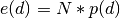$e(d) = N * p(d)$ where N is the total number of observed distances and p is the probability for spot distance d. The probability p has been pre-calculated for each spot distance. The probabilities for intra-specific spot distances are from the model of Distribution for intra-specific spot distances and the probabilities for inter-specific distances are from the model of Distribution for inter-specific spot distances. The probabilities have been hard coded into the application:

Intra-specific spot distances:

Spot Distance	Probability
1	40/300
1.41	32/300
2	30/300
2.24	48/300
2.83	18/300
3	20/300
3.16	32/300
3.61	24/300
4	10/300
4.12	16/300
4.24	8/300
4.47	12/300
5	8/300
5.66	2/300

Inter-specific spot distances:

Spot Distance	Probability
0	25/625
1	80/625
1.41	64/625
2	60/625
2.24	96/625
2.83	36/625
3	40/625
3.16	64/625
3.61	48/625
4	20/625
4.12	32/625
4.24	16/625
4.47	24/625
5	16/625
5.66	4/625

Depending on the analysis, the records matching the species selection are first grouped by positive spots number (analysis “Attraction within Species”) or by ratios group (analysis “Attraction between Species”). See section Record Grouping.

Each row for the results of the Chi-squared tests contains the results of a single test on a spots/ratios group. Each row can have the following elements:

Positive Spots: A number representing the number of positive spots. For this test only records matching that number of positive spots were used.
Ratios Group: A number representing the ratios group. For this test only records grouped in that ratios group were used.
n (plates): The number of plates that match the number of positive spots.
n (distances): The number of spot distances derived from the records matching the positive spots number.
P-value: The P-value for the test.
Chi squared: The value the Chi-squared test statistic.
df: The degrees of freedom of the approximate chi-squared distribution of the test statistic.
Mean Observed: The mean of the observed spot distances. This is calculated separately.
Mean Expected: The mean of the expected spot distances. This is calculated separately.
Remarks: A summary of the results. Shows whether the p-value is significant, and if so, how significant and decides based on the means if the species attract (observed mean < expected mean) or repel (observed mean > expected mean).

Some spots/ratios groups might me missing from the list of results. This is because spots/ratios groups that don’t have matching records are skipped, so they are not displayed in the list of results.

Plate Areas Definition for Chi-squared Test¶

Describes the definition of the plate areas set with the Define Plate Areas dialog. See the description for that dialog to get the meaning of the letters A, B, C and D.

Species Totals per Plate Area for Chi-squared Test¶

Area ID: See the Plate Areas Definition for Chi-squared Test section of the report to see the definition of each area.
Observed Totals: How many times the selected species was found present in each of the plate areas.
Expected Totals: The expected totals for the selected species.

Summary Report¶

A summary report contains basic information from multiple standard reports. Such a summary report is basically a table where each row represents a single analysis and the columns contain the results per data group.

In the summary report a result is only displayed if one of the statistical tests done for a species (combination) was considered significant. Some statistical tests are repeated and in this case there is a p-value for each repeat. In this case the p-value is calculated with 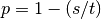$p = 1 - (s/t)$ where s is the number of significant p-values for the major form of significance. For example, if attraction was more often significant than rejection, then s is the total number of significant p-values for attraction. And t is the total number of repeats for the test. So with 20 repeats and $\alpha = 0.05$ , 19 out of 20 repeats must have had a significant p-value in one direction for the test result to be considered significant.

Below are the definitions for the result codes used in summary reports.

na: There is not enough data for the analysis or in case of the Chi Squared test one of the expected frequencies is less than 5.
s: The result for the statistical test was significant.
ns: The result for the statistical test was not significant.
pr: There was a significant preference for the plate area in question.
rj: There was a significant rejection for the plate area in question.
at: There was a significant attraction for the species in question.
rp: There was a significant repulsion for the species in question.

The summary report for each analysis are explained below.

Summary Report “Spot Preference”¶

Example report:

		Wilcoxon rank sum test								Chi-sq
Species	n (plates)	A	B	C	D	A+B	C+D	A+B+C	B+C+D	A,B,C,D
Obelia dichotoma	177	pr; p=0.0000	ns; p=1.0000	rj; p=0.0000	ns; p=0.0500	ns; p=0.3500	rj; p=0.0000	ns; p=1.0000	ns; p=1.0000	s; χ²=103.98; p=0.0000
Obelia geniculata	91	ns; p=0.4500	ns; p=1.0000	rj; p=0.0000	ns; p=0.1000	ns; p=1.0000	rj; p=0.0000	ns; p=1.0000	ns; p=1.0000	s; χ²=62.30; p=0.0000
Obelia longissima	341	pr; p=0.0000	ns; p=1.0000	rj; p=0.0000	rj; p=0.0000	pr; p=0.0000	rj; p=0.0000	ns; p=1.0000	rj; p=0.0000	s; χ²=435.22; p=0.0000

Explanation of the columns:

Species: Name of the species.
n (plates): The total number of plates for the species selection. The real number of plates used for each data group may be smaller. Use the “Save All” button to see the number of plates used for each data group.
A, B, C, D, A+B, C+D, A+B+C, and B+C+D: In this report the results are grouped by plate area (see Grouping by Plate Area). For the Wilcoxon rank sum test, the test is performed on each of the four plate areas, plus the combinations “A+B”, “C+D”, “A+B+C”, and “B+C+D”. For the Chi squared test the user defined plate areas are used. The user defined plate areas can be seen in the column name (e.g. “A+B,C,D” means that areas A and B were combined).

Summary Report “Attraction within Species”¶

Explanation of the columns:

Species: Name of the species.
n (plates): The total number of plates for the species selection. The real number of plates used for each data group may be smaller. Use the “Save All” button to see the number of plates used for each data group.
2-24, 2, 3, ..., 24: In this report the results are grouped by positive spot numbers (see Record grouping by number of positive spots).

Summary Report “Attraction between Species”¶

Example report:

			Wilcoxon rank sum test						Chi-squared test
Species A	Species B	n (plates)	1-5	1	2	3	4	5	1-5	1	2	3	4	5
Obelia dichotoma	Obelia geniculata	12	ns; p=0.8500	ns; p=0.0500	at; p=0.0000	ns; p=1.0000	na	na	ns; χ²=16.90; p=0.2615	rp; χ²=35.36; p=0.0013	at; χ²=38.12; p=0.0005	ns; χ²=7.21; p=0.9263	na	na
Obelia dichotoma	Obelia longissima	81	rp; p=0.0000	ns; p=0.1000	rp; p=0.0000	rp; p=0.0000	rp; p=0.0000	rp; p=0.0000	rp; χ²=420.68; p=0.0000	rp; χ²=134.34; p=0.0000	rp; χ²=164.86; p=0.0000	rp; χ²=170.01; p=0.0000	rp; χ²=96.88; p=0.0000	rp; χ²=43.53; p=0.0001
Obelia geniculata	Obelia longissima	39	rp; p=0.0000	ns; p=0.9500	ns; p=0.9500	ns; p=0.5500	ns; p=0.9500	rp; p=0.0000	rp; χ²=211.92; p=0.0000	rp; χ²=39.46; p=0.0003	rp; χ²=28.69; p=0.0115	rp; χ²=105.26; p=0.0000	ns; χ²=8.14; p=0.8821	rp; χ²=141.94; p=0.0000

In this example the columns containing numbers (1,2,..) represent

Explanation of the columns:

Species A: Name of the first species.
Species B: Name of the species the first species was compared with.
n (plates): The total number of plates for the species selection. The real number of plates used for each data group may be smaller. Use the “Save All” button to see the number of plates used for each data group.
1-5, 1, 2, 3, 4, 5: In this report the results are grouped by positive spot ratio groups (see Record grouping by ratios groups).

Record Grouping¶

SETLyze performs statistical tests to determine the significance of results. The key statistical tests used to determine significance are the Wilcoxon rank-sum test and Pearson’s Chi-squared test. The tests are performed on records data that match the locations and species selection. It is however not a good idea to just perform the test on all matching records. For this reason the matching records are first grouped by a specific property. The tests are then performed on each group.

Two methods for grouping records have been implemented. One is by positive spots number, and the other is by positive spots ratio. We’ll describe each grouping method below.

Grouping by Plate Area¶

This type of grouping is done for analysis “Spot Preference”. Each group is a plate area or a combination of plate areas. The following groups are defined:

Plate area A
Plate area B
Plate area C
Plate area D
Plate area A+B
Plate area B+C
Plate area A+B+C
Plate area B+C+D

For each group, the number of positive spots for all plates and that specific plate area are calculated. These make up the observed values.

Record grouping by number of positive spots¶

This type of grouping is done in the case of calculated spot distances for a single species (or multiple species grouped together) on SETL plates (analysis “Attraction within Species”).

A record has a maximum of 25 positive spots, so this results in a maximum of 25 record groups. Group 1 contains records with just one positive spot, group 2 contains records with two positive spots, et cetera. Records of group 1 and 25 are left out however. Group 1 is skipped because it is not possible to calculate spot distances for records with just one positive spot. And group 25 is excluded because a significance test on records of this group will always result in a p-value of 1. This makes sense, because both the observed and expected distances are based on records with 25 positive spots, which is a full SETL plate. As a result, the observed and expected spot distances will be exactly the same.

The test is also performed on a group with number -24. Of course there is no such thing as records with minus 24 positive spots. Actually, the minus sign should be read as “up to”. So this test is also performed on records with up to 24 positive spots. This means that the significance test will also be performed on records of all groups together. Note that records of group 1 will still be ignored.

The results of the significance tests are presented in rows. Each row contains the result of the test for one group. The “Positive Spots” column tells you to which group each result belongs.

Record grouping by ratios groups¶

This type of grouping is done in the case of calculated spot distances between two different (groups of) species (analysis “Attraction between Species”).

When dealing with two species, plate records are matched that contain both species. This means we can get a ratio for the positive spots for each matching SETL plate record. Consider Spot distances on SETL plate (inter specific) which visualizes a SETL plate with positive spots of species A and B. There are two positive spots of one species, and three positive spots of the other. That makes the ratio for this plate 2:3. The order of the species doesn’t matter here, so a ratio A:B is considered the same as ratio B:A. All records are grouped based on this ratio. We’ve defined five ratios groups:

Note

$c = comb(s)$: A function for generating a list of two-item combinations with replacement c from a sequence of numbers s. The two-item combinations are ratios (e.g. (2,3) = ratio 2:3).
$s = seq(start,end)$: A function for creating a sequence of numbers s from a number range starting with start and ending at end. For example $seq(1,6) = 1,2,3,4,5$

Ratios group 1:

$comb(seq(1,6))$ = (1, 1), (1, 2), (1, 3), (1, 4), (1, 5), (2, 2), (2, 3), (2, 4), (2, 5), (3, 3), (3, 4), (3, 5), (4, 4), (4, 5), (5, 5)

Ratios group 2:

$comb(seq(1,11)) - comb(seq(1,6))$ = (1, 6), (1, 7), (1, 8), (1, 9), (1, 10), (2, 6), (2, 7), (2, 8), (2, 9), (2, 10), (3, 6), (3, 7), (3, 8), (3, 9), (3, 10), (4, 6), (4, 7), (4, 8), (4, 9), (4, 10), (5, 6), (5, 7), (5, 8), (5, 9), (5, 10), (6, 6), (6, 7), (6, 8), (6, 9), (6, 10), (7, 7), (7, 8), (7, 9), (7, 10), (8, 8), (8, 9), (8, 10), (9, 9), (9, 10), (10, 10)

Ratios group 3:

$comb(seq(1,16)) - comb(seq(1,11))$ = (1, 11), (1, 12), (1, 13), (1, 14), (1, 15), (2, 11), (2, 12), (2, 13), (2, 14), (2, 15), (3, 11), (3, 12), (3, 13), (3, 14), (3, 15), (4, 11), (4, 12), (4, 13), (4, 14), (4, 15), (5, 11), (5, 12), (5, 13), (5, 14), (5, 15), (6, 11), (6, 12), (6, 13), (6, 14), (6, 15), (7, 11), (7, 12), (7, 13), (7, 14), (7, 15), (8, 11), (8, 12), (8, 13), (8, 14), (8, 15), (9, 11), (9, 12), (9, 13), (9, 14), (9, 15), (10, 11), (10, 12), (10, 13), (10, 14), (10, 15), (11, 11), (11, 12), (11, 13), (11, 14), (11, 15), (12, 12), (12, 13), (12, 14), (12, 15), (13, 13), (13, 14), (13, 15), (14, 14), (14, 15), (15, 15)

Ratios group 4:

$comb(seq(1,21)) - comb(seq(1,16))$ = (1, 16), (1, 17), (1, 18), (1, 19), (1, 20), (2, 16), (2, 17), (2, 18), (2, 19), (2, 20), (3, 16), (3, 17), (3, 18), (3, 19), (3, 20), (4, 16), (4, 17), (4, 18), (4, 19), (4, 20), (5, 16), (5, 17), (5, 18), (5, 19), (5, 20), (6, 16), (6, 17), (6, 18), (6, 19), (6, 20), (7, 16), (7, 17), (7, 18), (7, 19), (7, 20), (8, 16), (8, 17), (8, 18), (8, 19), (8, 20), (9, 16), (9, 17), (9, 18), (9, 19), (9, 20), (10, 16), (10, 17), (10, 18), (10, 19), (10, 20), (11, 16), (11, 17), (11, 18), (11, 19), (11, 20), (12, 16), (12, 17), (12, 18), (12, 19), (12, 20), (13, 16), (13, 17), (13, 18), (13, 19), (13, 20), (14, 16), (14, 17), (14, 18), (14, 19), (14, 20), (15, 16), (15, 17), (15, 18), (15, 19), (15, 20), (16, 16), (16, 17), (16, 18), (16, 19), (16, 20), (17, 17), (17, 18), (17, 19), (17, 20), (18, 18), (18, 19), (18, 20), (19, 19), (19, 20), (20, 20)

Ratios group 5:

$comb(seq(1,25)) - comb(seq(1,21))$ = (1, 21), (1, 22), (1, 23), (1, 24), (2, 21), (2, 22), (2, 23), (2, 24), (3, 21), (3, 22), (3, 23), (3, 24), (4, 21), (4, 22), (4, 23), (4, 24), (5, 21), (5, 22), (5, 23), (5, 24), (6, 21), (6, 22), (6, 23), (6, 24), (7, 21), (7, 22), (7, 23), (7, 24), (8, 21), (8, 22), (8, 23), (8, 24), (9, 21), (9, 22), (9, 23), (9, 24), (10, 21), (10, 22), (10, 23), (10, 24), (11, 21), (11, 22), (11, 23), (11, 24), (12, 21), (12, 22), (12, 23), (12, 24), (13, 21), (13, 22), (13, 23), (13, 24), (14, 21), (14, 22), (14, 23), (14, 24), (15, 21), (15, 22), (15, 23), (15, 24), (16, 21), (16, 22), (16, 23), (16, 24), (17, 21), (17, 22), (17, 23), (17, 24), (18, 21), (18, 22), (18, 23), (18, 24), (19, 21), (19, 22), (19, 23), (19, 24), (20, 21), (20, 22), (20, 23), (20, 24), (21, 21), (21, 22), (21, 23), (21, 24), (22, 22), (22, 23), (22, 24), (23, 23), (23, 24), (24, 24)

Ratios where one species has covered all 25 spots are excluded from this group because the p-value would be insignificant for such ratios.

You can imagine that the results of the statistical test performed on records from ratios group 1 has a higher reliability than the results for ratios group 5. Records from ratios group 1 have fewer positive spots. Finding that species A is often close to species B on records of group 5 doesn’t say much. The high number of positive spots naturally results in spots sitting close to each other. This is however not the case for records of group 1, where there is enough space for the species to sit. Finding them next to each other in group 1 probably means something.

The significance test is also performed on ratios group with number -5. This group includes ratios from all 5 groups (still excluding ratios with 25).

The results of the significance tests are presented in rows. Each row contains the result of the test for one group. The “Ratios Group” column tells you to which group each result belongs.

Exporting SETL data from the Access database¶

Export to CSV files¶

This section describes how to export the SETL data from the Microsoft Access database to CSV files.

Open the SETL database file (*.mdb) in Microsoft Access. You’ll see four tables in the left column: SETL_localities, SETL_plates, SETL_records and SETL_species.
To export a table, right-click on it to open the drop menu. From the menu select Export > Text file. Then give the filename of the output file. Make sure to include the table name in the filename (e.g. setl_localities.csv for the “SETL_localities” table). Uncheck all other options and press OK.
In the next dialog that appears select the option that separates fields with a character. The separator character must be a semicolon (”;”). If it’s not, change it by clicking the Advanced button. Then click Finish to export the data to a CSV file.
Repeat steps 2 and 3 for all tables.
You should end up with four files, one CSV file for each table. Put these files in one folder.

Export to Excel files¶

The database tables can also be exported to Excel files. Only the import of Excel 97/2000/XP/2003 (*.xls) files are supported by SETLyze, so be sure to select the right format.

Use Cases¶

Possible use cases which describe how SETLyze can be used to find answers to biological questions regarding the settlement of species on SETL plates.

Use Cases for SETLyze
- Use Case 1: Spot Preference
- Use Case 2: Attraction of Species (intra-specific)