Testing and Optimization

This document describes the steps taken to test and optimize SETLyze.

Testing

Calculation of expected spot distances

Analyses 2 and 3 have a built-in consistency check. In all cases must the number of calculated expected spot distances be equal to the number of observed spot distances. If this is not the case, than this indicates a bug in the application. This is what the check looks like:

# Perform a consistency check. The number of observed and
# expected spot distances must always be the same.
count_observed = len(observed)
count_expected = len(expected)
if count_observed != count_expected:
    raise ValueError("Number of observed and expected spot "
        "distances are not equal. This indicates a bug "
        "in the application.")

Testing spot distances for normal distribution

This part describes the method used to test if the spot distances on a SETL-plate follow a standard normal distribution. The choice of the statistical tests used for some analyis is based on the results of this test. This is because some statistical tests assume that the samples follow a normal distribution while some do not.

First step was to calculate the probabilities for the spot distances on a SETL-plate. A Python script was written to calculate the probabilities for all possible spot distances on a single SETL-plate. This was done for both intra-specific and inter-specific spot distances. The results were then loaded into R and visualised in a histogram (see Distribution for intra-specific spot distances and Distribution for inter-specific spot distances).

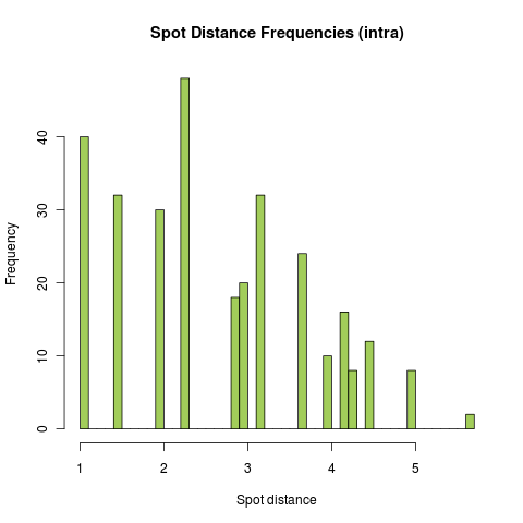
Distribution for intra-specific spot distances

The frequencies were obtained by calculating all possible distances between two spots if all 25 spots are covered. The same test was done with different numbers of positive spots randomly placed on a plate with 100.000 repeats. All resulting distributions are very similar to this figure.

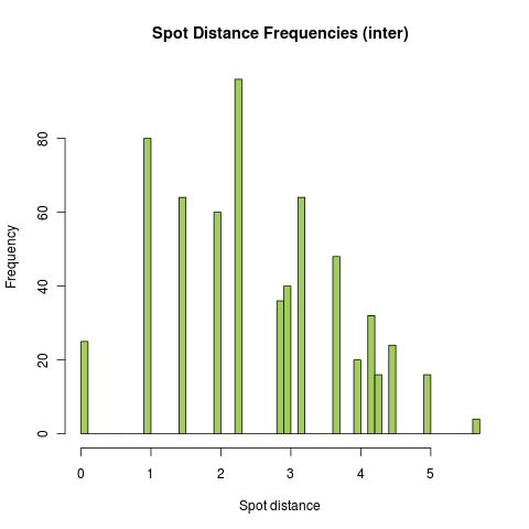
Distribution for inter-specific spot distances

The frequencies were obtained by calculating all possible distances between two spots with ratio 25:25 (species A and B have all 25 spots covered). The same test was done with different positive spots ratios (spots randomly placed on a plate, 100.000 repeats). All resulting distributions are very similar to this figure.

The histograms show that there is a tendency towards a normal distrubution, but this is obstructed because of the limited number of possible spot distances. To test if the distribution of spot distances really don’t follow a standard normal distribution, we performed the One-sample Kolmogorov-Smirnov test on both (intra and inter) spot distance samples. This was again done with the use of R. The results are as follows:

> ks.test(dist_intra[,1], 'pnorm', mean=mean(dist_intra[,1]), sd=sd(dist_intra[,1]))

    One-sample Kolmogorov-Smirnov test

data:  dist_intra[, 1]
D = 0.1419, p-value = 1.133e-05
alternative hypothesis: two-sided

Warning message:
In ks.test(dist_intra[, 1], "pnorm", mean = mean(dist_intra[, 1]),  :
  cannot compute correct p-values with ties

> ks.test(dist_inter[,1], 'pnorm', mean=mean(dist_inter[,1]), sd=sd(dist_inter[,1]))

    One-sample Kolmogorov-Smirnov test

data:  dist_inter[, 1]
D = 0.1188, p-value = 4.403e-08
alternative hypothesis: two-sided

Warning message:
In ks.test(dist_inter[, 1], "pnorm", mean = mean(dist_inter[, 1]),  :
  cannot compute correct p-values with ties

So the p-values can’t be correctly computed which might render the results unreliable. So the Shapiro-Wilk normality test was performed as well:

> shapiro.test(dist_intra[, 1])

    Shapiro-Wilk normality test

data:  dist_intra[, 1]
W = 0.9512, p-value = 1.955e-08

> shapiro.test(dist_inter[, 1])

    Shapiro-Wilk normality test

data:  dist_inter[, 1]
W = 0.9725, p-value = 1.957e-09

Again very low p-values are found, which is why we assume that spot distances on a SETL-plate don’t follow a standard normal distribution. Hence we chose the Wilcoxon rank-sum test because this test doesn’t assume that data come from a normal distribution (Dalgaard). Welch’s t-test is an adaptation of Student’s t-test (Wikipedia). And because Student’s t-test does assume that data come from a normal distribution (Dalgaard), we chose not to use this test.

Optimization

Spot distance calculation

It was thought that retrieving pre-calculating spot distances from a table in the local database would be faster than calculating each spot distance on run time. Python’s timeit module was used to find out which method is faster. For this purpose a small script was written:

#!/usr/bin/env python

import os
import timeit
from sqlite3 import dbapi2 as sqlite

import setlyze.std

connection = sqlite.connect(os.path.expanduser('~/.setlyze/setl_local.db'))
cursor = connection.cursor()

test_record = [1,1,1,1,1,1,1,1,1,1,1,1,1,1,1,1,1,1,1,1,1,1,1,1,1]

def test1():
    """Get pre-calculated spot distances from the local database."""
    combos = setlyze.std.get_spot_combinations_from_record(test_record)

    for spot1,spot2 in combos:
        h,v = setlyze.std.get_spot_position_difference(spot1,spot2)
        cursor.execute( "SELECT distance "
                         "FROM spot_distances "
                         "WHERE delta_x = ? "
                         "AND delta_y = ?",
                         (h,v))
        distance = cursor.fetchone()

def test2():
    """Calculate spot distances on run time."""
    combos = setlyze.std.get_spot_combinations_from_record(test_record)

    for spot1,spot2 in combos:
        h,v = setlyze.std.get_spot_position_difference(spot1,spot2)
        distance = setlyze.std.distance(h,v)

# Time both tests.
runs = 1000
t = timeit.Timer("test1()", "from __main__ import test1")
print "test1: %f seconds" % (t.timeit(runs)/runs)

t = timeit.Timer("test2()", "from __main__ import test2")
print "test2: %f seconds" % (t.timeit(runs)/runs)

cursor.close()
connection.close()

The first test in the script gets pre-calculated spot distances from the database and the second test calculates spot distances on run time. The output was as follows:

test1: 0.011350 seconds
test2: 0.003097 seconds

This shows that calculating spot distances on run time is almost 4 times faster than retrieving pre-calculated spot distances from the database. So the use of the “spot_distances” table was dropped and spot distances are now calculated on run time.